What are GANs?

It stands for Generative-Adversarial Networks. Consists of two neural networks contesting against each other. These GANs can be used to generate real looking pictures and videos of virtually anything.

Two contesting neural networks are known as:

• Generative Network or Generator: Maximizes probability of fake data being classified as real. Tries to fool discriminator.
• Discriminative network or Discriminator : Generates probability that data is genuine. Classifies output of generator.

Training a GAN

1. Start with set of real data point as well as noisy data
2. Train discriminator to label real as real and fake as fake
3. Generate new noise points
4. Train generator to produce data that fools the discriminator
5. repeat using optimizer
6. Optimizer(Loss Functions) needed for both networks

Generating MNIST digits using a Simple GAN in Pytorch

Import Libraries

import os
import numpy as np
import matplotlib.pyplot as plt

import torch
import torchvision
import torch.nn as nn

from torchvision import transforms
from torchvision.utils import save_image

Preparing Data and applying transformations

batch_size = 10

device = torch.device('cuda' if torch.cuda.is_available() else 'cpu')

transform = transforms.Compose([
                transforms.ToTensor(),
                transforms.Normalize((0.5,), (0.5,))])

mnist = torchvision.datasets.MNIST(root='datasets/',
                                   train=True,
                                   transform=transform,
                                   download=True)

data_loader = torch.utils.data.DataLoader(dataset=mnist,
                                          batch_size=batch_size, 
                                          shuffle=True)

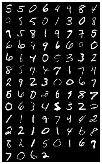
Visualizing Data

images, labels = iter(data_loader).next()

img = torchvision.utils.make_grid(images)

img = img.detach().numpy()
img = img.clip(0,1)

plt.figure(figsize = (12,10))
plt.imshow(np.transpose(img, (1,2,0)))
plt.axis('off')
plt.show()

Output(real):

Defining Networks and Hyper-parameters

latent_size = 64
hidden_size = 256
image_size = 784
num_epochs = 100

D = nn.Sequential(
    nn.Linear(image_size, hidden_size),
    nn.LeakyReLU(0.2),
    nn.Dropout(0.5),
    nn.Linear(hidden_size, hidden_size),
    nn.LeakyReLU(0.2),
    nn.Dropout(0.5),
    nn.Linear(hidden_size, 1),
    nn.Sigmoid())

G = nn.Sequential(
    nn.Linear(latent_size, hidden_size),
    nn.ReLU(),
    nn.Linear(hidden_size, hidden_size),
    nn.ReLU(),
    nn.Linear(hidden_size, image_size),
    nn.Tanh())

moving models to CUDA device if any

D = D.to(device)
G = G.to(device)

Training

bce_loss = nn.BCELoss()

d_optimizer = torch.optim.Adam(D.parameters(), lr=0.0002)
g_optimizer = torch.optim.Adam(G.parameters(), lr=0.0002)

total_step = len(data_loader)

for epoch in range(num_epochs):

    for i, (images, _) in enumerate(data_loader):

        images = images.reshape(batch_size, -1).to(device)

        # Create the labels which are later used as input for the BCE loss
        real_labels = torch.ones(batch_size, 1).to(device)
        fake_labels = torch.zeros(batch_size, 1).to(device)

        # Training the Discriminator

        # Compute BCE_Loss using real images where BCE_Loss(x, y): - y * log(D(x)) - (1-y) * log(1 - D(x))

        outputs = D(images)

        # Second term of the loss is always zero since real_labels == 1
        # This is what causes it to minimize the loss for real images
        d_loss_real = bce_loss(outputs, real_labels)
        real_score = outputs

        # Compute BCELoss using fake images

        z = torch.randn(batch_size, latent_size).to(device)
        fake_images = G(z)

        outputs = D(fake_images)

        # First term of the loss is always zero since fake_labels == 0
        # This is what causes it to maximize the loss for fake images
        d_loss_fake = bce_loss(outputs, fake_labels)
        fake_score = outputs

        # Backprop and optimize
        d_loss = d_loss_real + d_loss_fake

        d_optimizer.zero_grad()
        g_optimizer.zero_grad()

        d_loss.backward()
        d_optimizer.step()

        # Training the Generator

        # Compute loss with fake images

        z = torch.randn(batch_size, latent_size).to(device)
        fake_images = G(z)
        outputs = D(fake_images)

        # train G to maximize log(D(G(z)) instead of minimizing log(1-D(G(z)))

        g_loss = bce_loss(outputs, real_labels)

        # Backprop and optimize
        d_optimizer.zero_grad()
        g_optimizer.zero_grad()

        g_loss.backward()
        g_optimizer.step()

        if (i+1) % 200 == 0:
                        print(f"Epoch [{epoch}/{num_epochs}], Step [{i+1}/{total_step}], d_loss: {d_loss.item():.4f}, g_loss: {g_loss.item():.4f}, D(x): {real_score.mean().item():.2f}, D(G(z)): {fake_score.mean().item():.2f}")


    fake_images = fake_images.reshape(fake_images.size(0), 1, 28, 28)

Final Loss after training for 10 epochs

Epoch [9/10], Step [600/600], d_loss: 0.5627, g_loss: 2.8629, D(x): 0.79, D(G(z)): 0.17

Visualizing Outputs

img = torchvision.utils.make_grid(fake_images)

img = img.detach().cpu().numpy()
img = img.clip(0,1)

plt.figure(figsize = (12, 10))
plt.imshow(np.transpose(img, (1, 2, 0)))
plt.axis('off')
plt.show()

Output (fake mnist):

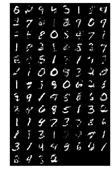
Training the network will take some time depending on the number of epochs you train for and device used for training.

Although, it was a very simple example of a GAN, more complex networks and models can be used to get better results.

Thanks a lot for Reading :)